
Mathematical Modeling in the School Curriculum
Presentation by Zalman Usiskin The University of Chicago at Teachers College, Columbia University, 26 Sep 2011

I would like to start with a true story – one of my favorite mathematical modeling stories. I call it "Mitchell's Golf Problem" after my first cousin Mitchell, who posed it to me on May 15, 1970.
In the afternoon of that day, I had learned that my mother died. At the time I was in my first year on the faculty of the University of Chicago and living on the far south side of Chicago. My parents lived on the north side about 45 minutes away. As soon as I learned of her sudden death, I informed my colleagues that I would not be around for a week; they said they would cover my classes, and I went to my apartment to get some changes of clothing because I knew I would be staying the entire next week with my father. And that evening Mitchell came over with other close relatives to console us. He knew that I would not have that much to do for the week and it would be good to take my mind off the loss, and so he told me his problem.
He said, "I golf with a group of 40 men every Saturday. We go off in foursomes; the first four guys to show up go out first, then the next four, and so on. The problem is that the same guys tend to come early every week, and other guys tend to come late. People are complaining that they are always golfing with the same people and never get to golf with most of the others. I am the secretary of the group and they asked me to form a schedule whereby every man would be in a foursome with every other person by the end of the summer."
Mitchell is no dummy. He went on, “I tried to figure this out but every process I tried wound up collapsing after a few weeks well before guys had played with everyone.” I immediately responded that this problem was right up my alley and I would try for a solution in 13 weeks, the minimum. Mitchell said he did not need such an optimal solution because there were many more weeks than that over a season. He said, “If I could have a schedule with everyone playing with everyone else even in 19 or 20 weeks, that would be great.
As soon as I had some free time, I went at the problem. I put down the numbers from 1 to 40 in 4 columns.
| 1 | 2 | 3 | 4 |
| 5 | 6 | 7 | 8 |
| 9 | 10 | 11 | 12 |
| 13 | 14 | 15 | 16 |
| 17 | 18 | 19 | 20 |
| 21 | 22 | 23 | 24 |
| 25 | 26 | 27 | 28 |
| 29 | 30 | 31 | 32 |
| 33 | 34 | 35 | 36 |
| 37 | 38 | 39 | 40 |
Here were my foursomes for the first week. Now what should I do for the second week? Perhaps go down the columns. So foursomes for the second week became 1, 5, 9, 13; 17, 21, 25, 29; 33, 37, 2, 6; and so on. This worked for a few weeks but then it started to give me people playing with each other twice even in the first five weeks. Maybe go diagonal: 1, 6, 11, 16; 5, 10, 15, 20; etc. I wound up in the same place as Mitchell, a little frustrated. This was not as simple a problem as I had thought.
To make a long story short – though if you want, during the question period I will tell you the longer story – I was unable to find a solution in 13 weeks. But I did find a solution in 15 weeks, and I mailed it to Mitchell. A short time later I received a call from him. He was very happy. He had taken my solution and worked up a schedule and sent it to all the members of the golfing group, and they were happy, too. But he said that he had to modify my solution in two ways. First, there were 41 golfers in the group, not 40. Second, there are these two men who hate each other and will not play with one another. He said, “I modified the solution by making myself the 41st player. Every week there is someone who is on vacation or sick and cannot make it, and I will just take that person's place. And I switched some people so that the two guys who hate each other would never be in the same foursome.
The Modeling Process
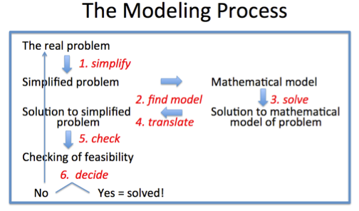
Mitchell's Golf Problem exemplifies the modeling process. Modeling starts with a real problem. The first step in the process is simplifying the problem, which Mitchell did by converting 41 to 40 and ignoring the fact that two men would not play together. I have indicated the steps by arrows. The next step is translating the simplified problem into mathematics (i.e., finding a mathematical model). The third step is to work with the mathematics – in this case the mathematics of block design. Then, once a solution has been found to the mathematical problem, there is the step of translating the solution back to the original situation, and then asking whether the solution is feasible. In advance Mitchell knew that my solution would not be feasible, but he had a way of making it feasible. If there had been no feasible solution, say no way to get everyone playing with each other even in 19 or 20 weeks, Mitchell would have had to go back perhaps even to the beginning of the problem, maybe replacing 40 by 41, maybe looking for a solution whereby over a 2-year period each man would have played with every other.
The mathematical modeling of Mitchell's problem began as soon as I denoted the golfers by the numbers 1 through 40. This enabled me to apply mathematical operations to obtain the needed foursomes. Even this step is not obvious to people who are not into mathematics; a well-educated friend of mine was surprised I did not keep people’s names in the mix. This would have made a difficult real problem even more difficult.
We Model All the Time!
Mathematical modeling is not an arcane activity, or one that only professionals do. It is so common that it is incumbent on us to understand what modeling can do and what pitfalls we should try to avoid. Teachers, in particular, come into contact with modeling in a variety of ways.
- A student obtains a score on a test, typically a single number. This score is on some scale, and that scale is a mathematical model that ostensibly describes how much the student knows of what has been tested. In terms of the modeling process, the problem to model is that we want to know how much the student knows about a certain area. This is an impossible task, so we simplify the problem by selecting a few things we think are important and asking what the student knows about these things. We assign weights of importance to each thing we have selected, and we decide to add the weights to get a single number representing what the student knows of this area. All of this is getting a mathematical model of what the student knows. The student takes the test and we do some calculations to get a single number. This is the mathematical solution. Now we have to translate that into the real world, often to give a letter grade. And so we do. But we have to look at the feasibility of this grade. Did too many students fail based on the model we used? If so, we deem the model as unsuitable and we may wish to curve the test – that is, to change the model. And we do the same thing at the end of each grading period; that is, we create a model that we hope accurately indicates performance, we work with that model, and – unless we are quite rigid, we look at the grades that the model gives us and test those grades for feasibility and accuracy. Are the students we think know the most getting the highest grades? You get the idea.
- In business and economics, value-added models have become common. This is an attempt to measure the worth of something by mathematically comparing a scenario before a treatment is undertaken and the scenario after the treatment and asking how much the treatment influenced the change. Some people want to evaluate teachers based on a value-added model. This is very controversial because the translation of the real school world into the model requires an extraordinary simplification of the real situation, namely a simplification that ignores the effects of student attitudes and abilities.
- A third type of model is commonly treated in school mathematics, but not viewed as modeling. How big is an object? We have lots of mathematical ways to answer that question. Consider an airplane. We might describe its size by its length, its wingspan, its height off the ground, its weight, the maximum weight it can handle, and the maximum number of passengers it can handle, and maybe you can think of a few more. We recognize that you cannot describe an airplane’s size by a single number.
- And yet some people believe you can describe a person’s mental capacity by a single number – IQ. Could anything be as foolish? But it is the simplicity of a single number, the attractiveness of a single number that has us use single numbers to determine all sorts of things, from the batting champion in the major leagues to comparing the educational systems of different countries.
Geometric Mathematical Models
I needn’t tell you that scale models of buildings and manufactured objects are geometric models. Most photographs are 2-dimensional models of 3-dimensional situations. We work with these models to determine information about the actual situation and translate what we have found back to the situation. For this, ratio and proportions are exceedingly important, and we see the applications of similarity and projections.
We use geometric models in algebra. We teach that the path of a ball thrown by a person or hit by a bat or golf club, or the path of a bullet from a rifle or a gun, and more generally that the path of any projectile – an object that is thrown, or shot – is a parabola. And we know that a parabola can be described by a quadratic equation.
The parabola may be thought of as a mathematical model, a geometric model of the actual situation, for the path of a projectile is not really a parabola. In order to exactly be a parabola, the force of gravity would have to be constant, there would have to be no wind or other force acting on the projectile, and there would have to be no spin. In baseball it is not just curveballs that curve, but almost all pitches. Paths of batted balls can be affected quite a bit by the wind. If you have seen golf on television lately, you will have seen the latest technology that tracks the path of a golf shot from the tee. Rarely are these paths straight. All these paths, in fact, are rarely coplanar. So we assume that there is no spin, no wind, and constant gravity.
We make assumptions in physical situations for the same reason that Mitchell made the assumption in his golf problem of 40 golfers, not 41. To treat the actual path of a projectile is very difficult, and a description or interpretation of a simplified path is good enough for many purposes. It tells us, that under ideal circumstances, the peak height of a fly ball in baseball is halfway between the batter and the fielder who catches it, something that would surprise many people, for it is a common belief that a ball comes down in a path that is more vertical than it goes up. And by assuming the path is a parabola, we can also estimate – reasonably closely – how far a home run would have traveled had it not been stopped by seats in the bleachers. And I needn't tell you that before the days of heat-seeking and other projectiles that can change course in flight, calculating the path of a parabola from a few bits of information was important in warfare.
Three Types of Mathematical Models
I like to distinguish three types of mathematical models.
Some models are exact models, either because they are based on counting or iteration, or because the application arose from the mathematics, not the other way around. For example, compound interest is defined from a mathematical formula; it arises from the mathematics. Similarly, lotteries are merely mathematical games played with people. The Cost C in cents of mailing a letter first-class in the United States weighing n ounces is given exactly for 1 ≤ n ≤ 3.5 by the formula C = 44 + 17[n – 1]. A network of airplane routes provides a geometric example. Exact models are isomorphic to real situations. While this kind of use of mathematics is not always considered to be modeling, because there is no testing, estimation, or feasibility questions as found with other kinds of modeling, it is an important type of modeling that provides a grounding for other “messier” situations.
A second kind of model is the almost-exact theory-based model often found in applications to the physical world. A football is kicked and travels to a height of 40 feet and lands 50 yards from where it was kicked; describe its path. In the postage example just mentioned, avoid the greatest integer function and use C = 17n + 27. Find the volume of a can given its dimensions; it seems like it might be exact except for the errors in measurement, but in fact, few cans are exact cylinders. An oven is heated from room temperature to 350°; how does its temperature change over time? In these cases, from assumptions made about the situation, the mathematical model can be deduced. The assumptions usually presume an exactness that is not possible in the situation; measurement error, the necessity of rounding, statistical variability, and other factors force the model to be only an approximation of reality. Though some error is known to exist, a person can still trust to some extent the results obtained by using the model. These kinds of models are the ones most found in mathematics textbooks.
The third kind of model is the impressionistic model, a model that seems to fit a real situation but which is derived from no hard theory. For instance, here is a graph of the world record for running a mile, from 1913 to 1981.

The record over time looks linear. But of course the trend cannot be linear forever, since then at some time a runner would finish the mile before he started. Here the record is linear for two reasons: first, because it is a record, the function relating year and time must be a decreasing function; second, any smooth curve that would fit such a function would be linear when viewed over only a short period of time. It happens that even the 68 years of this record is a short period of time. You might use this graph to extrapolate for a few years, but not to go well into this century. A good model does not just describe; it also predicts.
I hesitate to say that much research in education and other social sciences fits linear models to data – you know this if you have ever studied linear regression – and in most situations there is no causal rationale for a linear model. The model may work for the given data but not be generalizable to any other data.
The perils of extrapolation are amply seen in this upload from Wikipedia http://upload.wikimedia.org/wikipedia/en/4/49/Manhattan_population.png of the population of Manhattan for 210 years.

Here the graph looks like that of an exponential function from 1790 through 1910, and as you know we often view population growth as exponential, but any prediction made in 1910 based on that model would have gone the wrong way! So would a prediction made in 1930 based on the preceding 20 years, or a prediction made in 1950, or one in 1980.
When we fit a function to data, as in the mile record or Manhattan population situations, it is very important to point out that we are working from assumptions about the situation that may be inaccurate or just very rough approximations.
Some models fit between the almost exact – theory based models and the impressionistic models. Among these are the models relating current test scores to future performance. Yes, we know there is a strong positive correlation, but there is no causation and there can be major exceptions to any trend that might be established.
Teaching Mathematical Modeling
In the 1970s I received an NSF grant to develop a first-year algebra course through applications. At the time, what constituted applications in algebra classes were problems that began like these: "A child is half as old as her father was…"; You have 19 quarters and dimes in your pocket…"; "I am thinking of a 3-digit number…"
As a person with a background in pure mathematics, I had little idea what I was going to do in this course, but I did come in with a basic idea: many of the traditional word problems in algebra were not applications nor did they teach students anything about applied mathematics. They were not applications because so many were what E.L. Thorndike (who everyone in this room should know about because he spent virtually his entire academic career as a Teachers College faculty member) called “reverse given-find” problems. That is, in order to make up the problem you had to know the answer. How would you know that you had 19 quarters and dimes in your pocket with a total value of $3.70 if you had not the opportunity to count the quarters and count the dimes?
The idea of reverse given-find is found throughout mathematics and it leads to great questions – given the roots of a polynomial equation, find the equation; given the area of a rectangle, find its possible dimensions, etc. But in real-world situations, these kinds of questions are typically rather phony.
The problem this poses for the teaching of mathematical modeling is that some students see nothing else but these kinds of phony or quasi-phony problems. They leave algebra and many of their mathematics classes without a clue as to why they are studying this content. Why is it required for graduation? Why is this on tests? Do I really need to know this mathematics?
This leads us to the first of two basic reasons why students cannot apply mathematics well. They have not been taught the applications. And it starts with arithmetic, where there is so much emphasis in the early grades on counting and not enough on measuring, and no mention of scales of any kind usually until algebra with the Fahrenheit-Celsius conversion formula. The second reason students cannot apply algebra is that, beyond applications with small whole numbers, they cannot apply the arithmetic that the algebra generalizes.
Consider the properties of multiplication that we teach. Multiplication is commutative. It is associative. It distributes over addition. 1 is the multiplicative identity. The reciprocal of a is 1/a and, more generally, the reciprocal of x/y is y/x. And, if you ask people what multiplication means or what multiplication is, they may say, "It's repeated addition."
As I think everyone in this room knows, repeated addition does not work if one is trying to explain 2/3 × 4/5, or 35% of $150. You can multiply if you are in a grocery store, buy 6 cans of beans, each of which costs 89¢, and want to find their total value. But that is not a multiplication situation; it is an addition situation, and multiplication is only a shortcut. For addition and subtraction, students learn some key words such as total or take-away, but they have no key words for multiplication. As a consequence, many students leave school not having any sort of concept about the possible uses of multiplication. As a result, students have to memorize formulas such as d = rt or A = lw without realizing that these formulas result from essential uses of multiplication.
If we refer to the modeling diagram, we see that this analysis exposes a gap in the curriculum of many students. There is little or no instruction in the finding of the mathematical model. Students have no place to turn except to memorize without understanding.
We thus began a practice that, I am happy to say, has been picked up in a variety of ways by curricula at all levels K–12. That practice is to emphasize, in a quasi-formal way, the connections between the real world and mathematical operations. While this has been done forever for some applications of addition and subtraction, with putting-together and take-away, even those ideas do not cover all the important uses of those operations, and overall, the connections are not discussed enough in a systematic way.
These days, with the common core standards, there is much rhetoric about "learning progressions." So here is a learning progression with respect to mathematical modeling. We begin with uses of numbers. In primary school, we expect that students have seen numbers used as counts and as measures. In these uses, we deal not just with numbers but with quantities, which are numbers and their associated labels: counts have counting units and measures have units of measure. Students may also have seen that, in situations with two directions, positive and negative numbers arise. Fractions and percent show that numbers are also the result of ratio comparisons, and such numbers do not have units. π is a wonderful example of an irrational number used as a ratio comparison Numbers also represent locations. Street addresses, rank orders, and scales such as the Celsius scale for temperatures or the decibel scale for sound intensity represent this fourth use of numbers. Numbers also may be used as identification or codes, as in charge card numbers or ISBNs. And of course there are numbers simply used as numbers, such as when we examine prime numbers or lucky numbers.
The uses of the operations of arithmetic are associated with some but not all of the uses of numbers. The sum x + y has meaning if x and y are counts or measures, but not necessarily when x and y are ratio comparisons, and almost never if x and y are codes. You do not add the scales of two maps, nor do you add your telephone numbers. Also, when x and y are locations such as scale values, the sum x + y does not have much meaning. For example, the sum of two temperatures does not have meaning. Yet, in these very same contexts, other operations may have meaning. The difference x – y of two temperatures almost always has a meaning. Two scales may be able to be multiplied to get the result of applying one scale after the other.
Each of the operations has fundamental meanings: addition as putting-together or slide; subtraction as take-away or comparison, and special cases of comparison are error and change. Multiplication is acting across (including area and its discrete counterpart being array), size change, or rate factor; division is rate or ratio; powering is growth or change of dimension. The meanings are related to each other just as the operations are: for examples, take-away undoes putting-together; size change undoes ratio.
Allow me a true story about what happens when people do not understand the relationships between uses of numbers and uses of operations. I was sitting on a plane flight some years ago next to a man who was reading a magazine titled "Light Metal Age." No, this was not a magazine about some rock groups that were not into heavy metal, it is a magazine devoted to the production and fabrication of metals such as aluminum and titanium. The gentleman and I struck up a conversation and I found out that he worked for Alusuisse, the Switzerland equivalent of our Alcoa. He had written an article for the European counterpart of “Light Metal Age” and he was now reading the English translation. This translation included, as you might expect, the conversion of metric units into our U.S. customary units, including the translation of Centigrade into Fahrenheit. In one place in the article, he noted an error in the translation. A particular process with aluminum needed to be done at a particular temperature with a 5°C leeway. Instead of realizing that temperatures are scale values, and a difference of 5°C is equivalent to a difference of 9°F, the difference of 5°C was translated as a 41°F leeway. Imagine a company thinking it had so much leeway in its production temperature only to find out that the translator treated scale values as if they were measures. Celsius and Fahrenheit are not units; they are names of scales.
Whereas the units of measures are usually ignored in the formulas students see in mathematics classrooms, they help to distinguish the various meanings of operations. Ratio division is when the divisor and dividend have the same units, and we say that the units cancel because the result is a ratio comparison. Rate division is when the divisor and dividend have different units. For instance, divide my height 5'10"or 70" by my weight, 170 lb, and you get a rate: 7/17 of a pound per inch. Divide the other way and you get an equivalent rate: 17/7 of an inch per pound. Or consider multiplication. With area or acting across multiplication, the units multiply to create a product unit: 4 boys×3 girls = 12 couples; inches×inches = square inches in area; kilowatts×hours = kilowatt-hours; etc. With size change, the magnitude of the size change – a scalar – is multiplied by a measure, and the result is a measure with the same unit, as in 20%×$600 = $120. In rate factor multiplication, as its name implies, one factor is a rate and the units multiply: For instance, Brooklyn has about 36,000 people per square mile. This is a rate. Multiply it by Brooklyn's area, about 70 square miles, and you get a good estimate of Brooklyn’s population, namely around 2,500,000.
I would be remiss if I did not mention that one of the earliest attempts to categorize the uses of the operations in this way was by Ethel Sutherland, in 1947, in her doctoral dissertation done at this institution.
As a progression, it is fundamentally important that in the primary school these uses of numbers and operations go beyond counts to include non-integers. Then, in the lower secondary school, these uses can be employed to give meaning to algebraic expressions. For instance, when items with unit costs x, y, and z are purchased in quantities A, B, and C, the sum Ax + By + Cz is an addition putting together rate-factor multiplications to arrive at a total price. In the calculation of the rate of change of a quantity at two different times, the numerator and denominator in the expression are subtraction comparisons and the division is a rate, so it is no surprise that the quotient represents a rate of change. Thus the idea of rate of change should precede the slope of a line, not follow it.
From the meanings of algebraic expressions come the situations that functions model. Linear functions arise from these linear combinations, or situations of constant increase or constant decrease. Exponential functions model situations of growth or decay. Quadratic functions model situations of acceleration or deceleration (the rate of a rate), or area. Trigonometric functions model circular motion and are often quite appropriate in situations where phenomena occur periodically. The broad kinds of situations that the various types of functions model should be as much a part of the curriculum as the mathematical properties of these functions, for it is almost certain we would not be studying these functions were it not for their applications.
Back to the Modeling Diagram
Let me restate this discussion of learning progressions in terms of the modeling diagram. Obviously a pivotal step in mathematical modeling is to find the model, that is, to find the mathematics that fits a particular situation. In much of school mathematics, this task has been dealt with by translating words describing the real situation into mathematics. This is why applications are so often categorized as "word problems." We have enough experience to know that this way of teaching modeling has very limited value. Word problems are highly stylized; applications are typically not restricted to a particular style.
Consequently, the finding of a mathematical model requires that a student recognize that a facet of the application situation is modeled by a corresponding facet of a particular mathematical idea or operation. To do this, the student needs a repertoire of the basic use ideas of mathematical concepts. In turn, obtaining that repertoire requires that when a mathematical concept is being studied, the student be introduced to its major uses. And, in fact, many curricula that teach mathematical modeling often introduce a mathematical idea by starting from a use. So, even though in the diagram, the mathematical modeling process goes from the real world situation to its mathematical counterpart, in order to teach mathematical modeling we must go in the reverse direction and study the basic uses of the mathematical ideas that are being discussed, because most important mathematical ideas have more than one basic use meaning. This is what makes them important.
Solving the Mathematical Problem
After finding a model, the next step in the modeling process is solving the problem as it has been restated in its mathematical model. Some people call this "doing the math." This is a difficult step for many students because in most classrooms in this country students are solving the problem in the mathematical model not because they really want to know something about the problem situation, but in order to practice some mathematical process. The application has not been there because it is important, but to provoke student interest in the mathematical idea and to disguise practice.
We know that the purpose is to deal with some mathematical process because in the real world, people use any technology they can to solve a problem, but in the classroom in the United States there is a feeling among many teachers that using technology is "cheating." It isn't cheating at all, but wisdom. All of this talk in the Common Core Standards about fluency – that is, speed and accuracy – is totally misguided. If you want fluency today, you use a calculator and computer. When do you see cashiers in a store use paper and pencil to add up how much it will cost you? When does the person who does your tax returns use paper and pencil when working on your return? In fact, if the cashiers or a tax preparer did use paper and pencil, would you gain or lose confidence in what they do?
There is not one mention of calculators in grades K–8 in the Common Core, and the use in high schools is limited to complicated expressions or explorations, not to the actual doing of everyday mathematics. This view is the opposite of the view towards technology in the real world and is just the opposite of what we need in this country to prepare students for today's workplace, let alone tomorrow's.
Turning to Geometry
So far my examples have been mainly from arithmetic and algebra. Let me now turn to geometry. How does geometry fit into all this? Very nicely, it happens.
In geometry, the basic notion is the point. "Point" is in most deductive systems an undefined term. This is not a weakness of mathematics, but a strength, because being undefined allows “point” to take on a variety of meanings. In particular, a point may be a location, an ordered pair or ordered triple or even an ordered n-tuple of numbers, a node of a network, or a dot. These notions of "point" are as basic as the uses of number, and just as uses of numbers lead us to uses of operations, so uses of points lead us to uses of lines. We might view discussion of these notions as the first step in a learning progression of modeling in geometry, but by this I do not mean that it should occur in that order. "Undefined term" is an advanced concept compared to these uses.
The mathematics of these various kinds of points is different. That is a basic reason why we have postulates. The postulates tell us what kinds of points and lines we are dealing with. For instance, there is the postulate that two distinct points determine a line; that is, there is exactly one line through two different points. This postulate holds for thinking of points as locations and ordered pairs, but does not hold for nodes in networks or dots.
I needn’t say much about the application of points as locations. This is the most common application of geometry, to objects in the plane or in space. We can describe these points also by ordered pairs. The postulates of plane Euclidean geometry fit our notion of point as location, and also as ordered pair in a rectangular coordinate system.
Just as we moved from number to operation, so we can move from point to line or curve.
Lines contain paths of shortest distances between points, and are subject to the postulates that connect points and lines. Curves contain other paths connecting points. We model objects by looking at their physical features and emulating those features in the models we study.
Points as ordered pairs, or ordered triples, or ordered n-tuples also have applications different from locations. In particular, data points may have any number of dimensions, and we often want to consider lines that fit these data points. As locations, n-dimensional points with n > 3 or n > 4 do not have much meaning, but data points with many dimensions are not at all uncommon.
Most of our geometry in school is done in the plane, and there is a subtlety to considering an ordered pair of real numbers as a conception of point. The graph of a function from the reals to the reals, the typical functions most studied in school, or, more generally, the graph of a set of ordered pairs, now becomes a geometric object, not just a representation of a function. So it has all the mathematical properties that we associate with lines and curves. Thus, for example, we can think of the graph of y = x2 not just as a representation of the quadratic function but as a geometric object.
Here the Common Core Standards are a great help. By prescribing that the definitions of congruence and similarity be in terms of transformations, they have opened the door for any figures to be considered in geometry, not just triangles, other polygons, and circles. So, for example, these curved arrows are all similar, and three of them are congruent. And these definitions apply as well to 3-space as to 2-space.

With the general conception of congruence and the ability to consider sets of ordered pairs as geometric figures, we can have theorems about graphs. One of these that is exemplified in many of today’s books is the Graph Translation Theorem: In a relation described by a sentence in x and y, the following two processes yield the same graph:
- replacing x by x – h and y by y – k;
- applying the translation T(x,y) = (x + h, y + k) to the graph of the original relation.
From this theorem, we can easily deduce that the graphs of any two exponential functions with the same base are congruent. Consider, for example, the graphs of y = 2x and y = 3 × 2x. Since we can write 3 as 2log23, we see that the graph of y = 2x is just the image of the graph of y = 3 × 2x under a horizontal translation of length log23. The implication of this result for modeling is that all phenomena that grow at the same rate – in this case double in a unit time period – follow the same growth curve, though they may start at different points on that curve.

The point as a node of a network is different from the point as a location or as an ordered pair of numbers. The postulates are not the same for networks; for instance, there may be two or more lines containing the same two points. A grid of airplane routes is an example. But there is still rich geometry here, started by Euler with the Konigsberg Bridge Problem and studied mainly in topology.
The fourth conception of point, that of a dot, may rankle some of you. A dot isn't a point, you may say, it is a representation of a point. Yes, a dot is a representation of a point when that point is thought of as a location, but it is very useful sometimes to think of the plane as a union of dots. In the screens in our televisions, computers and handheld devices, we call these points pixels.
In Chicago we have probably the most famous piece of art applying this conception, Seurat’s large canvas, Sunday Afternoon on the Island of La Grande Jatte (painted 1884-86), approximately 7 feet high and 10 feet wide, is an example of what artists call pointillism. Again the geometry is different; for instance, between two points there may not be a third point.

Knowing these alternate conceptions of points shows that it is not only Euclidean geometry that models the world, but other geometries as well. And notice how connected geometry and algebra become, and how the notion of a mathematical system – with its postulates, definitions, and theorems - that we so often associate only with pure mathematics becomes critical in the understanding of geometric modeling.
Analogies between Pure and Applied Mathematics
Applications are to applied mathematics as theoretical properties are to pure mathematics. More specifically, the use meanings of number and operations are to applied mathematics what the field properties of the real numbers are to pure mathematics. Combining rate and change to obtain the concept of rate of change is akin to combining postulates and definitions to obtain a theorem. The basic process by which we work with applications is mathematical modeling; the basic process by which we develop pure mathematics is that of proving.
We have been teaching (or trying to teach) students proof for quite a bit longer than we have been teaching modeling. What can we learn from that experience? Here are some thoughts.
- It is almost impossible to understand proofs with concepts that have just been introduced. For instance, the college student who is just introduced to the concept of group in abstract algebra finds it difficult to write proofs about groups immediately. Similarly, modeling in contexts not understood by students is likely to be a waste of time.
- The ability to do proofs in one domain does not necessarily extend to the ability to do proofs in another domain. The same is true for modeling. This suggests that students should learn a variety of types of modeling.
- Proof learning requires the language of if-then statements and justifying conclusions. Modeling requires the same logic – if these boundary conditions are assumed, then what can we deduce? Thus we should be able to use proof to teach modeling and use modeling to teach proof.
- Communication of proofs and modeling both require that students write using both mathematical and non-mathematical terminology. Independent of the mathematical concepts, the writing task itself poses difficulties for many students.
- Proof competence comes quite slowly. We should not expect modeling competence to come any more quickly.
- Some proofs, like the infinitude of primes or the irrationality of
 , are classic. Similarly, some models should be treated with the same reverence, and taught to all. One that would surely qualify is Kepler’s modeling of Tycho Brahe’s data about the orbits of the planets and coming up with what today are known as Kepler’s three laws, or the many applications of the normal curve in describing variability in a homogenous population.
Summary
In summary, we can say that the case for modeling as a standard part of the everyday experience in the mathematics classroom is grounded not only on the importance and motivational qualities of good applications, but also on the contributions that modeling and applications make to a deeper and richer understanding of mathematical concepts. However, in doing so I would urge that the sequence and selection of activities for mathematical modeling should be treated as carefully as we do the sequence and selection of activities for the pure mathematics that we have taught for generations.
Contact
UCSMP
1427 East 60th Street
Chicago, IL 60637
T: 773-702-1130
F: 773-834-4665
ucsmp@uchicago.edu
Connect
with other UCSMP users